Proud to be involved in the engineering in this project!
https://news.mit.edu/2020/peptide-drug-block-covid-19-cells-0327
Proud to be involved in the engineering in this project!
https://news.mit.edu/2020/peptide-drug-block-covid-19-cells-0327
It can be much simpler and much less error prone (user errors) to transform forces and moments between two points by using a cross product instead of using transformation matrices like:
The simple trick is to recognize that a cross product can be expressed as a matrix multiply as follows:
So to show how we would use the cross product to our advantage, see the the following example. We want to transform the forces and moments applied to a rigid body at point A to point B:
It’s quite easy to see that the forces along the cartesian coordinates remain the same between the two points, but the moments change due to the moment arm (ptb-pta).
It is also useful that displacements can be easily transformed using the transpose of the transformation matrix above:
This is an excerpt from Layton Hale’s lecture notes “Design and Analysis of Constraint Systems” from the November 2010 ASPE Conference.
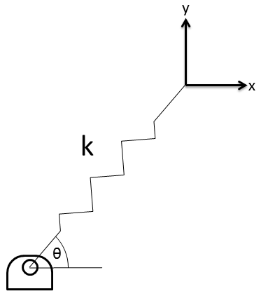
Many engineers make a simple mistake when determining the equivalent stiffness of a spring that is rotated with respect to a coordinate system. Typically they find and
, which are both incorrect.

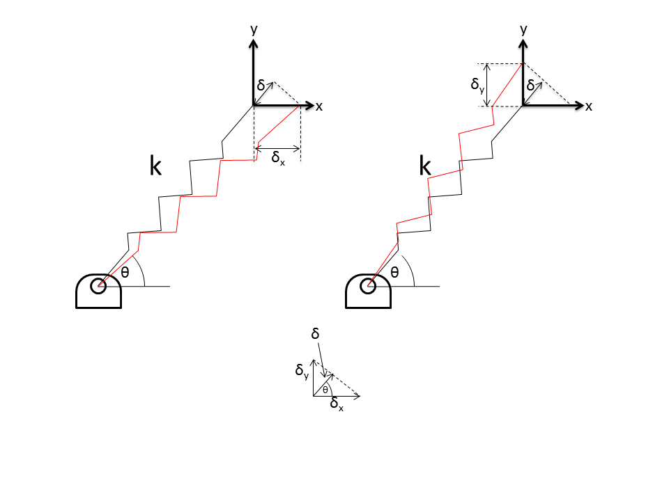
When we displace the spring in the x direction the compression of the spring along it’s axis is quite a bit less as you can see in the figure below. From the figures it is quite easy to see:
 It follows that the spring stiffness along the x-direction is:
We can then easily solve for the equivalent stiffness matrix as:
And now we can compute the forces along the rotated coordinate system as:
This is a continuation post on simple implementations of tuned-mass-dampers. For the curious please see my previous posts about TMDs here …
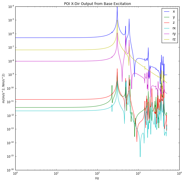
Say we have the 6-DOF model with frequency response as shown below. The FRF’s show the response of a leadscrew actuator to an acceleration disturbance at it’s base (continue reading about the leadscrew actuator here…). 
We can use a TMD to dampen the first few modes. As a first pass damper design, let’s set the mass ratio to be 10%. We then have
kg. Also, the first interesting system mode occurs around
hz, a general rule of thumb for determining the damper’s resonance is
. We then set
hz. It is trivial to determine the damper stiffness
. We can start with a damping value of
.
So we create a 6-DOF tuned-mass-damper by appending six 1-DOF TMD’s, and if so desired, each 1-DOF TMD can target different modes as they are independent of eachother.
The 6-DOF TMD is then feedback to the dynamic system and the resultant FRF’s are shown below. The dashed lines are the undamped and solid lines are the damped FRF’s. Notice the original resonance is quite suppressed, this will dramatically reduce the POI motion from base disturbances.
For further reading on tuned mass dampers can by Lei Zuo and Samir Nayfeh be found here.
I proposed using an improper transfer function to model a simple tuned-mass damper (read more here) with the transfer function:
To convert this to state-space representation we need to use the more generalized descriptor state-space notation which introduces the “E” term:
where ,
,
and
.
We derive as:
We then have the following states:
where
we can see that
On to fill out the rest of the matrices as:
where .
This python snippet is useful to reset the color cycle on matplotlib plots:
plt.gca().set_prop_cycle(None)
A client wanted to investigate adding a tuned mass damper (TMD) to their system to improve its performance. We developed a large FEA model to estimate the dynamics of the system and didn’t want to add the damper within the FEA model because it was quite large and long solve times prevented quick iteration. We came up with this simple method to estimate the impact a TMD would have on system performance.
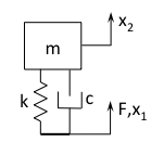
A 1-DOF tuned mass damper is easily derived from the diagram below

From the FEA model, we generated a state-space dynamic model that has a node at the location where we’d like to add the TMD. The input at that node is force (N, N.m) and the output at that node is displacement (m, rads). To incorporate the TMD into the dynamics all we need to do is apply the feedback loop as shown below:
To expand the TMD out to 6-DOF, we simply create six 1-DOF TMD’s and connect them to their respective inputs and outputs.
Now that the TMD dynamics are generated in post processing we can easily iterate on different designs (different masses, spring rates and damping values) to optimize the design. Frequency and transient responses are very quickly calculated as compared to solving FEA models.
For further reading on tuned mass dampers can by Lei Zuo and Samir Nayfeh be found here.