tuned mass damper

03Apr 2015

Tuned Mass Damper Applied to 6-DOF Model

This is a continuation post on simple implementations of tuned-mass-dampers. For the curious please see my previous posts about TMDs here …

Say we have the 6-DOF model with frequency response as shown below. The FRF’s show the response of a leadscrew actuator to an acceleration disturbance at it’s base (continue reading about the leadscrew actuator here…).

We can use a TMD to dampen the first few modes. As a first pass damper design, let’s set the mass ratio $\alpha=\frac{m_{damper}}{m_{sys}}$ to be 10%. We then have $m_{damper}=0.2$ kg. Also, the first interesting system mode occurs around $\omega_n=300$ hz, a general rule of thumb for determining the damper’s resonance is $\frac{\omega_{damper}}{\omega_{sys}}=\frac{1}{1-\alpha}$ . We then set $\omega_d = 278$ hz. It is trivial to determine the damper stiffness $k_{damper}=m_{damper}{\omega_d}^2$ . We can start with a damping value of $c=\frac{1}{2}m_{damper}\omega_d$ .

So we create a 6-DOF tuned-mass-damper by appending six 1-DOF TMD’s, and if so desired, each 1-DOF TMD can target different modes as they are independent of eachother.

$tmd_{6d} = \left[\begin{matrix}tmd_{1dx}\\tmd_{1dy}\\tmd_{1dz}\\tmd_{1drx}\\tmd_{1dry}\\tmd_{1drz}\end{matrix}\right]$

The 6-DOF TMD is then feedback to the dynamic system and the resultant FRF’s are shown below. The dashed lines are the undamped and solid lines are the damped FRF’s. Notice the original resonance is quite suppressed, this will dramatically reduce the POI motion from base disturbances.

For further reading on tuned mass dampers can by Lei Zuo and Samir Nayfeh be found here.

Posted in: Dynamics, Modeling, TMD ⋅ Tagged: Dynamics, Modeling, TMD

29Mar 2015

by Andrew Wilson

A client wanted to investigate adding a tuned mass damper (TMD) to their system to improve its performance. We developed a large FEA model to estimate the dynamics of the system and didn’t want to add the damper within the FEA model because it was quite large and long solve times prevented quick iteration. We came up with this simple method to estimate the impact a TMD would have on system performance.

A 1-DOF tuned mass damper is easily derived from the diagram below

$\frac{F}{x_{1}} = \frac{mcs^{3}+mks^{2}}{ms^{2}+cs+k}$

From the FEA model, we generated a state-space dynamic model that has a node at the location where we’d like to add the TMD. The input at that node is force (N, N.m) and the output at that node is displacement (m, rads). To incorporate the TMD into the dynamics all we need to do is apply the feedback loop as shown below:

To expand the TMD out to 6-DOF, we simply create six 1-DOF TMD’s and connect them to their respective inputs and outputs.

Now that the TMD dynamics are generated in post processing we can easily iterate on different designs (different masses, spring rates and damping values) to optimize the design. Frequency and transient responses are very quickly calculated as compared to solving FEA models.

For further reading on tuned mass dampers can by Lei Zuo and Samir Nayfeh be found here.

Posted in: Dynamics, Modeling ⋅ Tagged: Dynamics, Transfer Function, Tuned Mass Damper

03Apr 2015

Improper Transfer Function to State Space

by Andrew Wilson

I proposed using an improper transfer function to model a simple tuned-mass damper (read more here) with the transfer function:

$\frac{y}{u} = \frac{mcs^{3}+mks^{2}}{ms^{2}+cs+k}$

To convert this to state-space representation we need to use the more generalized descriptor state-space notation which introduces the “E” term:

$E\dot{x}(t)=Ax(t)+Bu(t)$

$y(t)=Cx(t)+Du(t)$

where $E,A \in \mathbb{R}^{n\times n}$ , $B \in \mathbb{R}^{n\times m}$ , $C \in \mathbb{R}^{p\times n}$ and $D \in \mathbb{R}^{p\times m}$ .

We derive $C$ as:

$y = C \times \left[\begin{matrix}x_1\\x_2\\x_3\\x_4\end{matrix}\right]$

$y = \left[\begin{matrix}mc,mk,0,0\end{matrix}\right]\times \left[\begin{matrix}x_1\\x_2\\x_3\\x_4\end{matrix}\right]$

We then have the following states:

$\left[\begin{matrix}x_1\\x_2\\x_3\\x_4\end{matrix}\right]=\left[\begin{matrix}us^3/d\\us^2/d\\us/d\\u/d\end{matrix}\right]$

$\left[\begin{matrix}\dot{x}_1\\\dot{x}_2\\\dot{x}_3\\\dot{x}_4\end{matrix}\right]=\left[\begin{matrix}us^4/d\\us^3/d\\us^2/d\\us/d\end{matrix}\right]$

where $d = ms^2+cs+k$

we can see that

$\begin{matrix}u&=&d\times x_4&\\u&=&ms^2x_4+csx_4+kx_4&\\u&=&m\dot{x}_3+cx_3+kx_4&\\\end{matrix}$

On to fill out the rest of the matrices as:

$\begin{matrix}E&\dot{X}&=&A&X&+&B&u\\ \left[\begin{matrix}0&1&0&0\\0&0&1&0\\0&0&m&0\\0&0&0&1\end{matrix}\right]&\left[\begin{matrix}\dot{x}_1\\\dot{x}_2\\\dot{x}_3\\\dot{x}_4\end{matrix}\right]&=&\left[\begin{matrix} 1&0&0&0\\0&1&0&0\\0&0&-c&-k\\0&0&0&1 \end{matrix}\right]&\left[\begin{matrix}x_1\\x_2\\x_3\\x_4\end{matrix}\right]&+&\left[\begin{matrix}0\\0\\1\\0\end{matrix}\right]&u\end{matrix}$

$\begin{matrix}Y&=&C&X&+&D&u&\\Y&=&\begin{matrix}\left[mc,mk,0,0\right]\end{matrix}&\left[\begin{matrix}x_1\\x_2\\x_3\\x_4\end{matrix}\right]&&\end{matrix}$

where $D=0$ .

Posted in: descriptor state space, Dynamics, Modeling, state space, transfer function ⋅ Tagged: Descriptor Model, Dynamics, Modeling, State Space, Transfer Function, Tuned Mass Damper

Modal + Servo Analysis

A client needed to determine the performance of a leadscrew actuator. A sensitive optical sensor quickly moves to various positions and holds very still once in position, even in the presence of external disturbances.

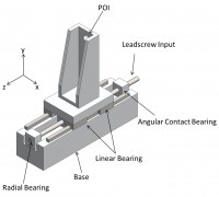
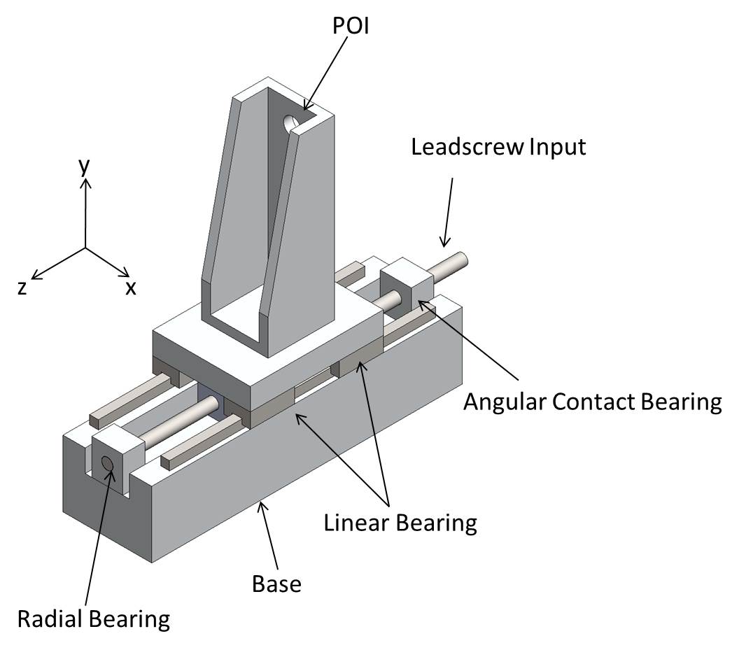
A simplified representation of the leadscrew actuator is shown below. A DC motor applies torque at the leadscrew, moving the carriage along the z-axis. In this particular case we are concerned with accurate positioning of the POI where a sensitive optical sensor is mounted. Note: in our simplified model, it is modeled as a hole.

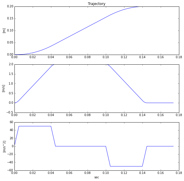
The position requirements are:

travel = 200 mm
velocity = 2 m/s
acceleration = 5 g ≈ 50 m/s²
jerk = 10,000 m/s³

Trajectory

And the base disturbances are summarized as:

Base Input Direction	0-10 Hz	10-500 Hz	500-5000 Hz
X-Dir [(nm/s²)²/hz]	0.11	25.0	0.01
Y-Dir [(nm/s²)²/hz]	0.15	50.0	0.01
Z-Dir [(nm/s²)²/hz]	0.14	30.0	0.01
RX-Dir [(nrad/s²)²/hz]	0.10	150.0	0.005
RY-Dir [(nrad/s²)²/hz]	0.10	70.0	0.005
RZ-Dir [(nrad/s²)²/hz]	0.10	15.0	0.005

The optical sensor must not exceed the stability requirements listed in the table below:

	X-Dir [μm]	Y-Dir [μm]	Z-Dir [μm]	Rx-Dir [μrad]	Ry-Dir [μrad]	Rz-Dir [μrad]
Stability Reqs.	1.0	1.0	1.0	5.0	5.0	5.0

First, the system mode shapes are calculated using FEA modal analysis:

Mode 1: This is a rigid body mode, screw rotation translates into carriage motion along the bearing. The lead of the screw dictates the motion.
Mode 2 & 3: In these two modes the leadscrew is bending in the horizontal and vertical planes. This is the first mode that would impact servo positioning performance. To improve the dynamics, we would need to design a stiffer leadscrew (larger diameter, shorter screw, etc.)
Mode 4, 5, 6: In these modes the carriage is rocking on the linear ball-guide bearings. To improve these dynamics some of the possibilities are:
- move carriage center-of-mass to the center of the bearings
- widen the bearing spacing
- lighten the carriage mass
- select stiffer bearings
- design a tuned mass damper to dampen these modes

Mode 1: 0 Hz	Mode 2: 229 Hz

Mode 3: 229 Hz	Mode 4: 306 Hz

Mode 5: 491 Hz	Mode 6: 504 Hz

Mode 7: 599 Hz	Mode 8: 629 Hz

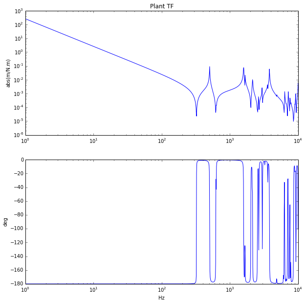
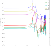
Once the mode shapes are calculated, we have the system Eigenvalues and Eigenvectors and can calculate the system state space model (ABCD matrices). The frequency response from torque input on the leadscrew to the screw rotation is shown below. Since the input and output are co-located the phase is always between 0 deg and -180 deg, quite easy to make a stable system.

Adding a simple lead controller with low pass filter get’s a crossover frequency of 75Hz and phase margin of 45 deg.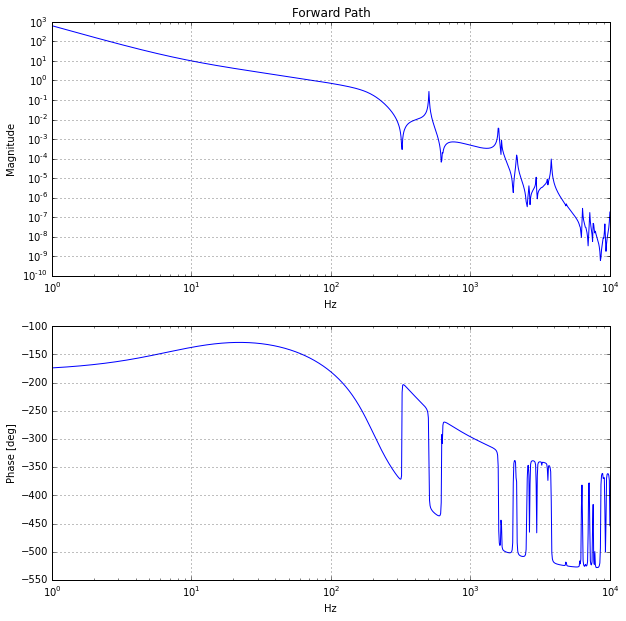

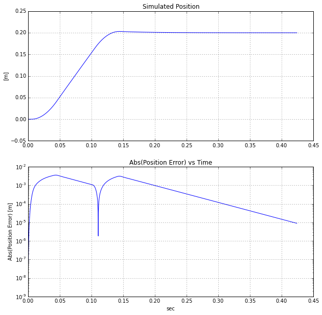
Now that we have the closed-loop model we can simulate the transient response as shown below:

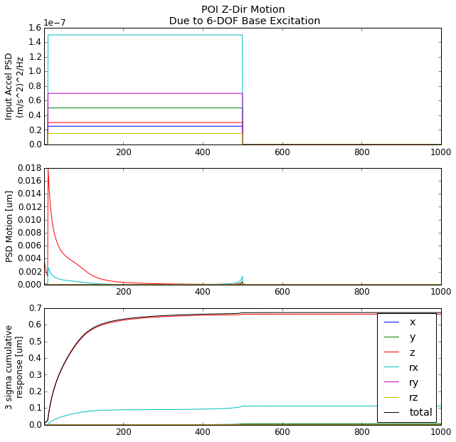
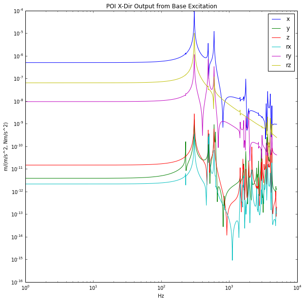
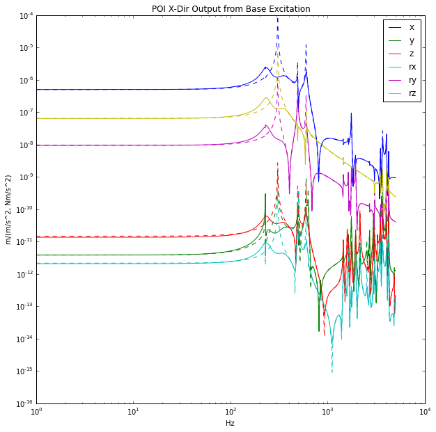
Below are the 6-DOF FRF’s for an input acceleration at the base of the machine and output motion at the poi.

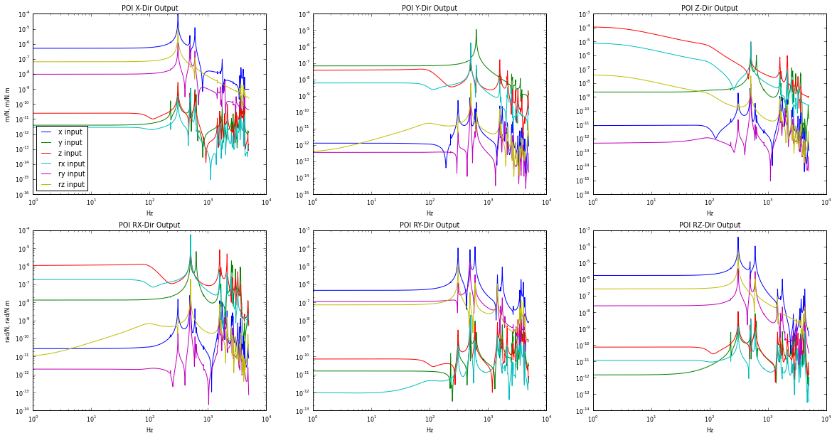
Given the base acceleration levels in the table above, we can estimate the motion of the poi.

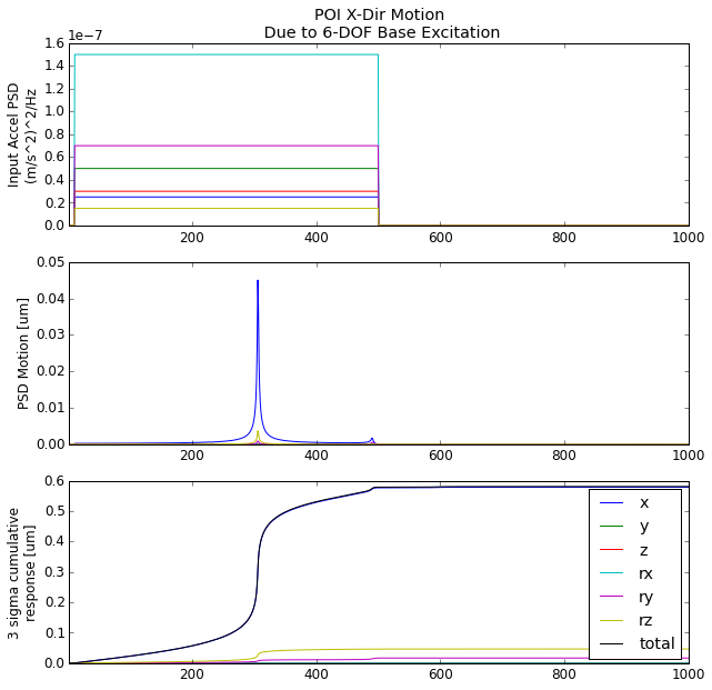
For X-dir motion of the POI, we can see that the mode at 302 Hz is the dominant contributor, and we should expect to see about 0.6 μm of motion.

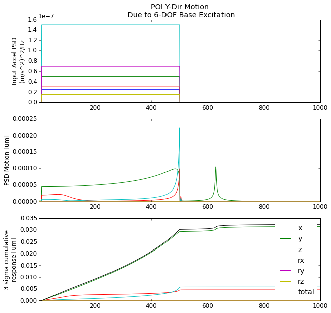
For Y-dir motion of the POI, we can see that most of the motion comes from the y-dir acceleration input across the 0-500Hz frequency range. Note, the mode at 629 Hz is excited but it doesn’t contribute much to the total motion. The “quasi-static” response of the system is the major contributor, if we need to reduce this motion, we should target stiffening the static stiffness in the y-dir. We should expect the POI to move about 0.03 μm due to the base excitation.

For Z-dir motion of the POI we expect to see approximately 0.65 μm motion, and this response is due to the quasi-static stiffness of the system in the z-direction.

For Rx-dir motion of the POI we expect to see about 0.25 μrad tilt and the major contributors are the quasi-static stiffness in the Z and RX direction.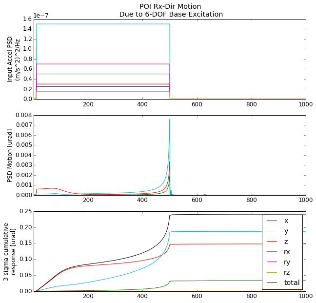

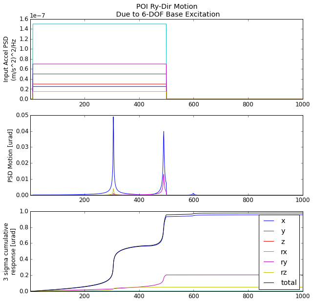
For Ry-dir motion of the POI we expect to see 1 μrad tilt and the major contributors are 306 Hz and 491 Hz modes excited by the X-direction base acceleration.

For Rz-dir motion of the POI we expect to see 2.25 μrad tilt and the major contributor is the 306 Hz mode excited by the X-direction base acceleration.

A summary of the results are in the table below. The system as modeled meets the desired requirements. We would suggest comparing the model to measured date to ensure accuracy. Also we suggest improving the X-dir and Z-dir stability of the system to have a bit more margin on meeting the requirements.

	X-Dir [μm]	Y-Dir [μm]	Z-Dir [μm]	Rx-Dir [μrad]	Ry-Dir [μrad]	Rz-Dir [μrad]
Stability Reqs.	1.0	1.0	1.0	5.0	5.0	50.0
Estimated Stability	0.60	0.03	0.65	0.25	1.0	2.25

Search Results: Tuned Mass Damper