A client wanted to investigate adding a tuned mass damper (TMD) to their system to improve its performance. We developed a large FEA model to estimate the dynamics of the system and didn’t want to add the damper within the FEA model because it was quite large and long solve times prevented quick iteration. We came up with this simple method to estimate the impact a TMD would have on system performance.
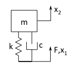
A 1-DOF tuned mass damper is easily derived from the diagram below
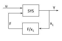
From the FEA model, we generated a state-space dynamic model that has a node at the location where we’d like to add the TMD. The input at that node is force (N, N.m) and the output at that node is displacement (m, rads). To incorporate the TMD into the dynamics all we need to do is apply the feedback loop as shown below:
To expand the TMD out to 6-DOF, we simply create six 1-DOF TMD’s and connect them to their respective inputs and outputs.
Now that the TMD dynamics are generated in post processing we can easily iterate on different designs (different masses, spring rates and damping values) to optimize the design. Frequency and transient responses are very quickly calculated as compared to solving FEA models.
For further reading on tuned mass dampers can by Lei Zuo and Samir Nayfeh be found here.

=Ax(t)+Bu(t)")
=Cx(t)+Du(t)")


![y = C \times \left[\begin{matrix}x_1\\x_2\\x_3\\x_4\end{matrix}\right]](https://s0.wp.com/latex.php?latex=y+%3D+C+%5Ctimes+%5Cleft%5B%5Cbegin%7Bmatrix%7Dx_1%5C%5Cx_2%5C%5Cx_3%5C%5Cx_4%5Cend%7Bmatrix%7D%5Cright%5D&bg=ffffff&fg=000000&s=0 "y = C \times \left[\begin{matrix}x_1\\x_2\\x_3\\x_4\end{matrix}\right]")
![y = \left[\begin{matrix}mc,mk,0,0\end{matrix}\right]\times \left[\begin{matrix}x_1\\x_2\\x_3\\x_4\end{matrix}\right]](https://s0.wp.com/latex.php?latex=y+%3D+%5Cleft%5B%5Cbegin%7Bmatrix%7Dmc%2Cmk%2C0%2C0%5Cend%7Bmatrix%7D%5Cright%5D%5Ctimes+%5Cleft%5B%5Cbegin%7Bmatrix%7Dx_1%5C%5Cx_2%5C%5Cx_3%5C%5Cx_4%5Cend%7Bmatrix%7D%5Cright%5D&bg=ffffff&fg=000000&s=0 "y = \left[\begin{matrix}mc,mk,0,0\end{matrix}\right]\times \left[\begin{matrix}x_1\\x_2\\x_3\\x_4\end{matrix}\right]")
![\left[\begin{matrix}x_1\\x_2\\x_3\\x_4\end{matrix}\right]=\left[\begin{matrix}us^3/d\\us^2/d\\us/d\\u/d\end{matrix}\right]](https://s0.wp.com/latex.php?latex=%5Cleft%5B%5Cbegin%7Bmatrix%7Dx_1%5C%5Cx_2%5C%5Cx_3%5C%5Cx_4%5Cend%7Bmatrix%7D%5Cright%5D%3D%5Cleft%5B%5Cbegin%7Bmatrix%7Dus%5E3%2Fd%5C%5Cus%5E2%2Fd%5C%5Cus%2Fd%5C%5Cu%2Fd%5Cend%7Bmatrix%7D%5Cright%5D&bg=ffffff&fg=000000&s=0 "\left[\begin{matrix}x_1\\x_2\\x_3\\x_4\end{matrix}\right]=\left[\begin{matrix}us^3/d\\us^2/d\\us/d\\u/d\end{matrix}\right]")
![\left[\begin{matrix}\dot{x}_1\\\dot{x}_2\\\dot{x}_3\\\dot{x}_4\end{matrix}\right]=\left[\begin{matrix}us^4/d\\us^3/d\\us^2/d\\us/d\end{matrix}\right]](https://s0.wp.com/latex.php?latex=%5Cleft%5B%5Cbegin%7Bmatrix%7D%5Cdot%7Bx%7D_1%5C%5C%5Cdot%7Bx%7D_2%5C%5C%5Cdot%7Bx%7D_3%5C%5C%5Cdot%7Bx%7D_4%5Cend%7Bmatrix%7D%5Cright%5D%3D%5Cleft%5B%5Cbegin%7Bmatrix%7Dus%5E4%2Fd%5C%5Cus%5E3%2Fd%5C%5Cus%5E2%2Fd%5C%5Cus%2Fd%5Cend%7Bmatrix%7D%5Cright%5D&bg=ffffff&fg=000000&s=0 "\left[\begin{matrix}\dot{x}_1\\\dot{x}_2\\\dot{x}_3\\\dot{x}_4\end{matrix}\right]=\left[\begin{matrix}us^4/d\\us^3/d\\us^2/d\\us/d\end{matrix}\right]")


![\begin{matrix}E&\dot{X}&=&A&X&+&B&u\\ \left[\begin{matrix}0&1&0&0\\0&0&1&0\\0&0&m&0\\0&0&0&1\end{matrix}\right]&\left[\begin{matrix}\dot{x}_1\\\dot{x}_2\\\dot{x}_3\\\dot{x}_4\end{matrix}\right]&=&\left[\begin{matrix} 1&0&0&0\\0&1&0&0\\0&0&-c&-k\\0&0&0&1 \end{matrix}\right]&\left[\begin{matrix}x_1\\x_2\\x_3\\x_4\end{matrix}\right]&+&\left[\begin{matrix}0\\0\\1\\0\end{matrix}\right]&u\end{matrix}](https://s0.wp.com/latex.php?latex=%5Cbegin%7Bmatrix%7DE%26%5Cdot%7BX%7D%26%3D%26A%26X%26%2B%26B%26u%5C%5C+%5Cleft%5B%5Cbegin%7Bmatrix%7D0%261%260%260%5C%5C0%260%261%260%5C%5C0%260%26m%260%5C%5C0%260%260%261%5Cend%7Bmatrix%7D%5Cright%5D%26%5Cleft%5B%5Cbegin%7Bmatrix%7D%5Cdot%7Bx%7D_1%5C%5C%5Cdot%7Bx%7D_2%5C%5C%5Cdot%7Bx%7D_3%5C%5C%5Cdot%7Bx%7D_4%5Cend%7Bmatrix%7D%5Cright%5D%26%3D%26%5Cleft%5B%5Cbegin%7Bmatrix%7D+1%260%260%260%5C%5C0%261%260%260%5C%5C0%260%26-c%26-k%5C%5C0%260%260%261+%5Cend%7Bmatrix%7D%5Cright%5D%26%5Cleft%5B%5Cbegin%7Bmatrix%7Dx_1%5C%5Cx_2%5C%5Cx_3%5C%5Cx_4%5Cend%7Bmatrix%7D%5Cright%5D%26%2B%26%5Cleft%5B%5Cbegin%7Bmatrix%7D0%5C%5C0%5C%5C1%5C%5C0%5Cend%7Bmatrix%7D%5Cright%5D%26u%5Cend%7Bmatrix%7D&bg=ffffff&fg=000000&s=0 "\begin{matrix}E&\dot{X}&=&A&X&+&B&u\\ \left[\begin{matrix}0&1&0&0\\0&0&1&0\\0&0&m&0\\0&0&0&1\end{matrix}\right]&\left[\begin{matrix}\dot{x}_1\\\dot{x}_2\\\dot{x}_3\\\dot{x}_4\end{matrix}\right]&=&\left[\begin{matrix} 1&0&0&0\\0&1&0&0\\0&0&-c&-k\\0&0&0&1 \end{matrix}\right]&\left[\begin{matrix}x_1\\x_2\\x_3\\x_4\end{matrix}\right]&+&\left[\begin{matrix}0\\0\\1\\0\end{matrix}\right]&u\end{matrix}")
![\begin{matrix}Y&=&C&X&+&D&u&\\Y&=&\begin{matrix}\left[mc,mk,0,0\right]\end{matrix}&\left[\begin{matrix}x_1\\x_2\\x_3\\x_4\end{matrix}\right]&&\end{matrix}](https://s0.wp.com/latex.php?latex=%5Cbegin%7Bmatrix%7DY%26%3D%26C%26X%26%2B%26D%26u%26%5C%5CY%26%3D%26%5Cbegin%7Bmatrix%7D%5Cleft%5Bmc%2Cmk%2C0%2C0%5Cright%5D%5Cend%7Bmatrix%7D%26%5Cleft%5B%5Cbegin%7Bmatrix%7Dx_1%5C%5Cx_2%5C%5Cx_3%5C%5Cx_4%5Cend%7Bmatrix%7D%5Cright%5D%26%26%5Cend%7Bmatrix%7D&bg=ffffff&fg=000000&s=0 "\begin{matrix}Y&=&C&X&+&D&u&\\Y&=&\begin{matrix}\left[mc,mk,0,0\right]\end{matrix}&\left[\begin{matrix}x_1\\x_2\\x_3\\x_4\end{matrix}\right]&&\end{matrix}")


