This is a continuation post on simple implementations of tuned-mass-dampers. For the curious please see my previous posts about TMDs here …
Say we have the 6-DOF model with frequency response as shown below. The FRF’s show the response of a leadscrew actuator to an acceleration disturbance at it’s base (continue reading about the leadscrew actuator here…). 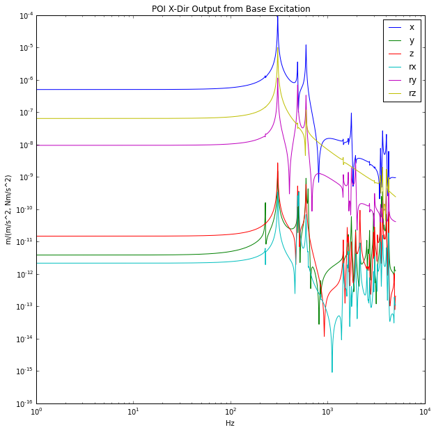
We can use a TMD to dampen the first few modes. As a first pass damper design, let’s set the mass ratio  to be 10%. We then have
  kg. Also, the first interesting system mode occurs around
  hz, a general rule of thumb for determining the damper’s resonance is
  . We then set
  hz. It is trivial to determine the damper stiffness
  . We can start with a damping value of
  .
.
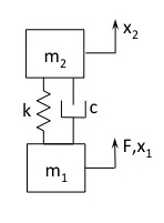
So we create a 6-DOF tuned-mass-damper by appending six 1-DOF TMD’s, and if so desired, each 1-DOF TMD can target different modes as they are independent of eachother.
![tmd_{6d} = \left[\begin{matrix}tmd_{1dx}\\tmd_{1dy}\\tmd_{1dz}\\tmd_{1drx}\\tmd_{1dry}\\tmd_{1drz}\end{matrix}\right]](https://s0.wp.com/latex.php?latex=tmd_%7B6d%7D+%3D+%5Cleft%5B%5Cbegin%7Bmatrix%7Dtmd_%7B1dx%7D%5C%5Ctmd_%7B1dy%7D%5C%5Ctmd_%7B1dz%7D%5C%5Ctmd_%7B1drx%7D%5C%5Ctmd_%7B1dry%7D%5C%5Ctmd_%7B1drz%7D%5Cend%7Bmatrix%7D%5Cright%5D&bg=ffffff&fg=000000&s=0 "tmd_{6d} = \left[\begin{matrix}tmd_{1dx}\\tmd_{1dy}\\tmd_{1dz}\\tmd_{1drx}\\tmd_{1dry}\\tmd_{1drz}\end{matrix}\right]")
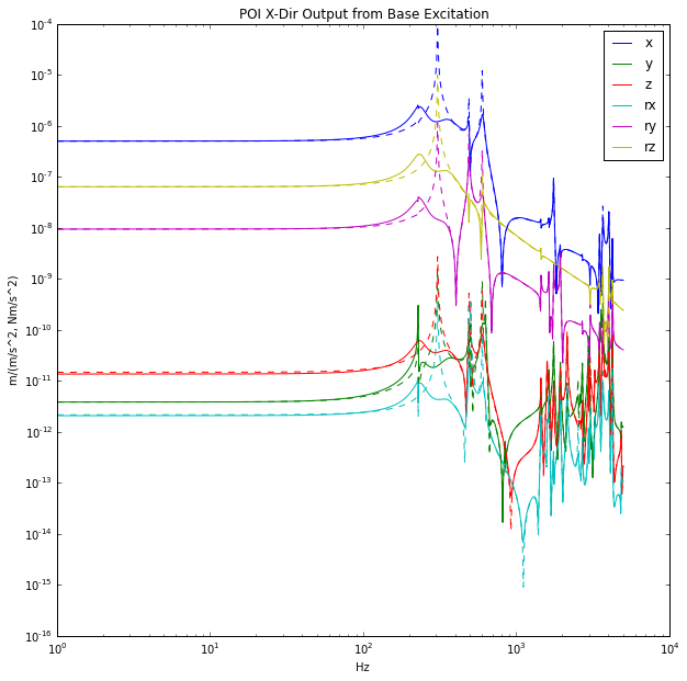
The 6-DOF TMD is then feedback to the dynamic system and the resultant FRF’s are shown below. The dashed lines are the undamped and solid lines are the damped FRF’s. Notice the original resonance is quite suppressed, this will dramatically reduce the POI motion from base disturbances.
For further reading on tuned mass dampers can by Lei Zuo and Samir Nayfeh be found here.


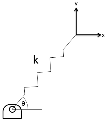


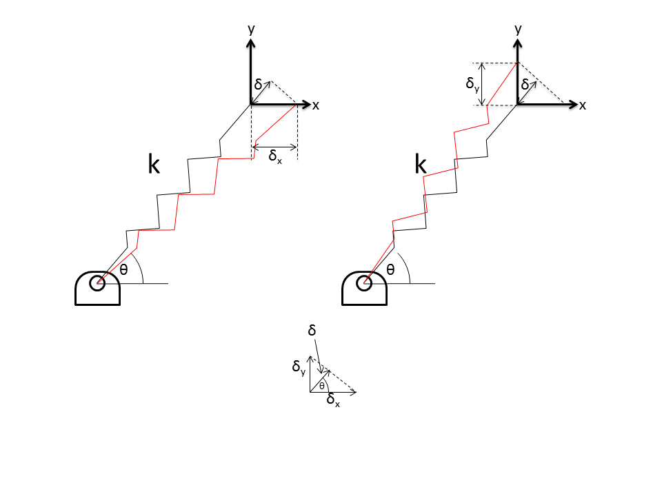 It follows that the spring stiffness along the x-direction is:


=Ax(t)+Bu(t)")
=Cx(t)+Du(t)")
 ,
,  ,
,  and
and  .
. as:
as:![y = C \times \left[\begin{matrix}x_1\\x_2\\x_3\\x_4\end{matrix}\right]](https://s0.wp.com/latex.php?latex=y+%3D+C+%5Ctimes+%5Cleft%5B%5Cbegin%7Bmatrix%7Dx_1%5C%5Cx_2%5C%5Cx_3%5C%5Cx_4%5Cend%7Bmatrix%7D%5Cright%5D&bg=ffffff&fg=000000&s=0 "y = C \times \left[\begin{matrix}x_1\\x_2\\x_3\\x_4\end{matrix}\right]")
![y = \left[\begin{matrix}mc,mk,0,0\end{matrix}\right]\times \left[\begin{matrix}x_1\\x_2\\x_3\\x_4\end{matrix}\right]](https://s0.wp.com/latex.php?latex=y+%3D+%5Cleft%5B%5Cbegin%7Bmatrix%7Dmc%2Cmk%2C0%2C0%5Cend%7Bmatrix%7D%5Cright%5D%5Ctimes+%5Cleft%5B%5Cbegin%7Bmatrix%7Dx_1%5C%5Cx_2%5C%5Cx_3%5C%5Cx_4%5Cend%7Bmatrix%7D%5Cright%5D&bg=ffffff&fg=000000&s=0 "y = \left[\begin{matrix}mc,mk,0,0\end{matrix}\right]\times \left[\begin{matrix}x_1\\x_2\\x_3\\x_4\end{matrix}\right]")
![\left[\begin{matrix}x_1\\x_2\\x_3\\x_4\end{matrix}\right]=\left[\begin{matrix}us^3/d\\us^2/d\\us/d\\u/d\end{matrix}\right]](https://s0.wp.com/latex.php?latex=%5Cleft%5B%5Cbegin%7Bmatrix%7Dx_1%5C%5Cx_2%5C%5Cx_3%5C%5Cx_4%5Cend%7Bmatrix%7D%5Cright%5D%3D%5Cleft%5B%5Cbegin%7Bmatrix%7Dus%5E3%2Fd%5C%5Cus%5E2%2Fd%5C%5Cus%2Fd%5C%5Cu%2Fd%5Cend%7Bmatrix%7D%5Cright%5D&bg=ffffff&fg=000000&s=0 "\left[\begin{matrix}x_1\\x_2\\x_3\\x_4\end{matrix}\right]=\left[\begin{matrix}us^3/d\\us^2/d\\us/d\\u/d\end{matrix}\right]")
![\left[\begin{matrix}\dot{x}_1\\\dot{x}_2\\\dot{x}_3\\\dot{x}_4\end{matrix}\right]=\left[\begin{matrix}us^4/d\\us^3/d\\us^2/d\\us/d\end{matrix}\right]](https://s0.wp.com/latex.php?latex=%5Cleft%5B%5Cbegin%7Bmatrix%7D%5Cdot%7Bx%7D_1%5C%5C%5Cdot%7Bx%7D_2%5C%5C%5Cdot%7Bx%7D_3%5C%5C%5Cdot%7Bx%7D_4%5Cend%7Bmatrix%7D%5Cright%5D%3D%5Cleft%5B%5Cbegin%7Bmatrix%7Dus%5E4%2Fd%5C%5Cus%5E3%2Fd%5C%5Cus%5E2%2Fd%5C%5Cus%2Fd%5Cend%7Bmatrix%7D%5Cright%5D&bg=ffffff&fg=000000&s=0 "\left[\begin{matrix}\dot{x}_1\\\dot{x}_2\\\dot{x}_3\\\dot{x}_4\end{matrix}\right]=\left[\begin{matrix}us^4/d\\us^3/d\\us^2/d\\us/d\end{matrix}\right]")


![\begin{matrix}E&\dot{X}&=&A&X&+&B&u\\ \left[\begin{matrix}0&1&0&0\\0&0&1&0\\0&0&m&0\\0&0&0&1\end{matrix}\right]&\left[\begin{matrix}\dot{x}_1\\\dot{x}_2\\\dot{x}_3\\\dot{x}_4\end{matrix}\right]&=&\left[\begin{matrix} 1&0&0&0\\0&1&0&0\\0&0&-c&-k\\0&0&0&1 \end{matrix}\right]&\left[\begin{matrix}x_1\\x_2\\x_3\\x_4\end{matrix}\right]&+&\left[\begin{matrix}0\\0\\1\\0\end{matrix}\right]&u\end{matrix}](https://s0.wp.com/latex.php?latex=%5Cbegin%7Bmatrix%7DE%26%5Cdot%7BX%7D%26%3D%26A%26X%26%2B%26B%26u%5C%5C+%5Cleft%5B%5Cbegin%7Bmatrix%7D0%261%260%260%5C%5C0%260%261%260%5C%5C0%260%26m%260%5C%5C0%260%260%261%5Cend%7Bmatrix%7D%5Cright%5D%26%5Cleft%5B%5Cbegin%7Bmatrix%7D%5Cdot%7Bx%7D_1%5C%5C%5Cdot%7Bx%7D_2%5C%5C%5Cdot%7Bx%7D_3%5C%5C%5Cdot%7Bx%7D_4%5Cend%7Bmatrix%7D%5Cright%5D%26%3D%26%5Cleft%5B%5Cbegin%7Bmatrix%7D+1%260%260%260%5C%5C0%261%260%260%5C%5C0%260%26-c%26-k%5C%5C0%260%260%261+%5Cend%7Bmatrix%7D%5Cright%5D%26%5Cleft%5B%5Cbegin%7Bmatrix%7Dx_1%5C%5Cx_2%5C%5Cx_3%5C%5Cx_4%5Cend%7Bmatrix%7D%5Cright%5D%26%2B%26%5Cleft%5B%5Cbegin%7Bmatrix%7D0%5C%5C0%5C%5C1%5C%5C0%5Cend%7Bmatrix%7D%5Cright%5D%26u%5Cend%7Bmatrix%7D&bg=ffffff&fg=000000&s=0 "\begin{matrix}E&\dot{X}&=&A&X&+&B&u\\ \left[\begin{matrix}0&1&0&0\\0&0&1&0\\0&0&m&0\\0&0&0&1\end{matrix}\right]&\left[\begin{matrix}\dot{x}_1\\\dot{x}_2\\\dot{x}_3\\\dot{x}_4\end{matrix}\right]&=&\left[\begin{matrix} 1&0&0&0\\0&1&0&0\\0&0&-c&-k\\0&0&0&1 \end{matrix}\right]&\left[\begin{matrix}x_1\\x_2\\x_3\\x_4\end{matrix}\right]&+&\left[\begin{matrix}0\\0\\1\\0\end{matrix}\right]&u\end{matrix}")
![\begin{matrix}Y&=&C&X&+&D&u&\\Y&=&\begin{matrix}\left[mc,mk,0,0\right]\end{matrix}&\left[\begin{matrix}x_1\\x_2\\x_3\\x_4\end{matrix}\right]&&\end{matrix}](https://s0.wp.com/latex.php?latex=%5Cbegin%7Bmatrix%7DY%26%3D%26C%26X%26%2B%26D%26u%26%5C%5CY%26%3D%26%5Cbegin%7Bmatrix%7D%5Cleft%5Bmc%2Cmk%2C0%2C0%5Cright%5D%5Cend%7Bmatrix%7D%26%5Cleft%5B%5Cbegin%7Bmatrix%7Dx_1%5C%5Cx_2%5C%5Cx_3%5C%5Cx_4%5Cend%7Bmatrix%7D%5Cright%5D%26%26%5Cend%7Bmatrix%7D&bg=ffffff&fg=000000&s=0 "\begin{matrix}Y&=&C&X&+&D&u&\\Y&=&\begin{matrix}\left[mc,mk,0,0\right]\end{matrix}&\left[\begin{matrix}x_1\\x_2\\x_3\\x_4\end{matrix}\right]&&\end{matrix}")
 .
.